Scaling GNNs via Neighbor Sampling
One of the challenges of Graph Neural Networks is to scale them to large graphs, e.g., in industrial and social applications. Traditional deep neural networks are known to scale well to large amounts of data by decomposing the training loss into individual samples (called a mini-batch) and approximating exact gradients stochastically. In contrast, applying stochastic mini-batch training in GNNs is challenging since the embedding of a given node depends recursively on all its neighbor’s embeddings, leading to high inter-dependency between nodes that grows exponentially with respect to the number of layers. This phenomenon is often referred to as neighbor explosion. As a simple workaround, GNNs are typically executed in a full-batch fashion (see here for an example), where the GNN has access to all hidden node representations in all its layers. However, this is not feasible in large-scale graphs due to memory limitations and slow convergence.
Scalability techniques are indispensable for applying GNNs to large-scale graphs in order to alleviate the neighbor explosion problem induced by mini-batch training, i.e. node-wise, layer-wise or subgraph-wise sampling techniques, or to decouple propagations from predictions. In this tutorial, we take a closer look at the most common node-wise sampling approach, originally introduced in the “Inductive Representation Learning on Large Graphs” paper.
Neighbor Sampling
PyG implements neighbor sampling via its torch_geometric.loader.NeighborLoader class.
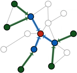
Neighbor sampling works by recursively sampling a fixed number of at most \(k\) neighbors for a node \(v \in \mathcal{V}\), i.e. \(\tilde{\mathcal{N}}(v) \subset \mathcal{N}(v)\) with \(|\tilde{\mathcal{N}}| \le k\), leading to an overall bounded \(L\)-hop neighborhood size of \(\mathcal{O}(k^L)\).
That is, starting from a set of seed nodes \(\mathcal{B} \subset \mathcal{V}\), we sample at most \(k\) neighbors for every node in \(v \in \mathcal{B}\), and then proceed to sample neighbors for every sampled node in the previous hop, and so on.
The resulting graph structure holds a directed \(L\)-hop subgraph around every node in \(v \in \mathcal{B}\), for which it is guaranteed that every node has at least one path of at most length \(L\) to at least one of the seed nodes in \(\mathcal{B}\).
As such, a message passing GNN with \(L\) layers will incorporate the full set of sampled nodes in its computation graph.
It is important to note that neighbor sampling can only mitigate the neighbor explosion problem to some extend since the overall neighborhood size still increases exponentially with the number of layers. As a result, sampling for more than two or three iterations is generally not feasible.
Often times, the number of sampled hops and the number of message passing layers is kept in sync.
Specifically, it is very wasteful to sample for more hops than there exist message passing layers since the GNN will never be able to incorporate the features of the nodes sampled in later hops into the final node representation of its seed nodes.
However, it is nonetheless possible to utilize deeper GNNs, but one needs to be careful to convert the sampled subgraph into a bidirectional variant to ensure correct message passing flow.
PyG provides support for this via an additional argument in NeighborLoader, while other mini-batch techniques are designed for this use-case out-of-the-box, e.g., ClusterLoader, GraphSAINTSampler and ShaDowKHopSampler.
Basic Usage
Note
In this section of the tutorial, we will learn how to utilize the Node2Vec class of PyG to train GNNs on single graphs in a mini-batch fashion.
A fully working example on large-scale real-world data is available in examples/reddit.py.
The NeighborLoader is initialized from a PyG Data or HeteroData object and defines how sampling should be performed:
input_nodesdefines the set of seed nodes from which we want to start sampling from.num_neighborsdefines the number of neighbors to sample for each node in each hop.batch_sizedefines the size of seed nodes we want to consider at once.replacedefines whether to sample with or without replacement.shuffledefines whether seed nodes should be shuffled at every epoch.
import torch
from torch_geometric.data import Data
from torch_geometric.loader import NeighborLoader

x = torch.randn(8, 32)  # Node features of shape [num_nodes, num_features]
y = torch.randint(0, 4, (8, ))  # Node labels of shape [num_nodes]
edge_index = torch.tensor([
    [2, 3, 3, 4, 5, 6, 7],
    [0, 0, 1, 1, 2, 3, 4]],
)

#   0  1
#  / \/ \
# 2  3  4
# |  |  |
# 5  6  7

data = Data(x=x, y=y, edge_index=edge_index)

loader = NeighborLoader(
    data,
    input_nodes=torch.tensor([0, 1]),
    num_neighbors=[2, 1],
    batch_size=1,
    replace=False,
    shuffle=False,
)
Here, we initialize the NeigborLoader to sample subgraphs for the first two nodes, where we want to sample 2 neighbors in the first hop, and 1 neighbor in the second hop.
Our batch_size is set to 1, such that input_nodes will be split into chunks of size 1.
In the execution of NeighborLoader, we expect that the seed node 0 samples nodes 2 and 3 in the first hop. In the second hop, node 2 samples node 5, and node 3 samples node 6.
Let’s confirm by looking at the output of the loader:
batch = next(iter(loader))

batch.edge_index
>>> tensor([[1, 2, 3, 4],
            [0, 0, 1, 2]])

 batch.n_id
 >>> tensor([0, 2, 3, 5, 6])

 batch.batch_size
 >>> 1
The NeighborLoader will return a Data object, which contains the following attributes:
batch.edge_indexcontain the edge indices of the subgraph.batch.n_idcontains the original node indices of all the sampled nodes.batch.batch_sizecontains the number of seed nodes/the batch size.
In addition, node and edge features will be filtered to only contain the features of sampled nodes/edges, respectively.
Importantly, batch.edge_index contains the sampled subgraph with relabeled node indices, such that its indices range from 0 to batch.num_nodes - 1.
If you want to reconstruct the original node indices of batch.edge_index, do:
batch.n_id[batch.edge_index]
>>> tensor([[2, 3, 5, 6],
            [0, 0, 2, 3]])
Furthermore, while NeighborLoader starts sampling from seed nodes, the resulting subgraph will hold edges that point to the seed nodes.
This aligns well with the default PyG message passing flow from source to destination nodes.
Lastly, nodes in the output of NeighborLoader are guaranteed to be sorted.
In particular, the first batch_size sampled nodes will exactly match with the seed nodes that were used for sampling:
batch.n_id[:batch.batch_size]
>>> tensor([0])
Afterwards, we can use NeighborLoader as a data loading routine to train GNNs on large-scale graphs in mini-batch fashion.
For this, let’s create a simple two-layer GraphSAGE model:
from torch_geometric.nn import GraphSAGE

device = torch.device('cuda' if torch.cuda.is_available() else 'cpu')

model = GraphSAGE(
    in_channels=32,
    hidden_channels=64,
    out_channels=4,
    num_layers=2
).to(device)

optimizer = torch.optim.Adam(model.parameters(), lr=0.01)
We can now combine the loader and model to define our training routine:
import torch.nn.functional as F

for batch in loader:
    optimizer.zero_grad()
    batch = batch.to(device)
    out = model(batch.x, batch.edge_index)

    # NOTE Only consider predictions and labels of seed nodes:
    y = batch.y[:batch.batch_size]
    out = out[:batch.batch_size]

    loss = F.cross_entropy(out, y)
    loss.backward()
    optimizer.step()
The training loop follows a similar design to any other PyTorch training loop.
The only important difference is that by default the model will output a matrix of shape [batch.num_nodes, *], while we are only interested in the predictions of the seed nodes.
As such, we can use efficient slicing both on the node predictions and the ground-truth information batch.y to only obtain predictions and ground-truth information of actual seed nodes.
This ensures that we are only making use of the first batch_size many nodes for loss and metric computation.
Hierarchical Extension
A drawback of Neighborloader is that it computes a representations for all sampled nodes at all depths of the network.
However, nodes sampled in later hops no longer contribute to the node representations of seed nodes in later GNN layers, thus performing useless computation.
NeighborLoader will be marginally slower since we are computing node embeddings for nodes we no longer need.
This is a trade-off we make to obtain a clean, modular and experimental-friendly GNN design, which does not tie the definition of the model to its utilized data loader routine.
The Hierarchical Neighborhood Sampling tutorial shows how to eliminate this overhead and speed up training and inference in mini-batch GNNs further.
Advanced Options
NeighborLoader provides many more features for advanced usage.
In particular,
NeighborLoadersupports both sampling on homogeneous and heterogeneous graphs out-of-the-box. For sampling on heterogeneous graphs, simply initialize it with aHeteroDataobject. Sampling on heterogeneous graphs viaNeighborLoaderallows for fine-granular control of sampling parameters, e.g., it allows to specify the number of neighbors to sample for each edge type individually. Take a look at the Heterogeneous Graph Learning tutorial for additional information.By default,
NeighborLoaderfuses sampled nodes across different seed nodes into a single subgraph. This way, shared neighbors of seed nodes will not be duplicated in the resulting subgraph and hence save memory. You can disable this behavior by passing thedisjoint=Trueoption to theNeighborLoader.By default, the subgraphs returned from
NeighborLoaderwill be directed, which restricts its use to GNNs with equal depth to the number of sampling hops. If you want to utilize deeper GNNs, specify thesubgraph_typeoption. If set to"bidirectional", sampled edges are converted to bidirectional edges. If set to"induced", the returned subgraph will contain the induced subgraph of all sampled nodes.NeighborLoaderis designed to perform sampling from individual seed nodes. As such, it is not directly applicable in a link prediction scenario. For this use-cases, we developed theLinkNeighborLoader, which expects a set of input edges, and will return subgraphs that were created via neighbor sampling from both source and destination nodes.