Point Cloud Processing
This tutorial explains how to leverage Graph Neural Networks (GNNs) for operating and training on point cloud data. Although point clouds do not come with a graph structure by default, we can utilize PyG transformations to make them applicable for the full suite of GNNs available in PyG. The key idea is to create a synthetic graph from point clouds, from which we can learn meaningful local geometric structures via a GNN’s message passing scheme. These point representations can then be used to, e.g., perform point cloud classification or segmentation.
3D Point Cloud Datasets
PyG provides several point cloud datasets, such as the PCPNetDataset, S3DIS and ShapeNet datasets.
To get started, we also provide the GeometricShapes dataset, which is a toy dataset that contains various geometric shapes such cubes, spheres or pyramids.
Notably, the GeometricShapes dataset contains meshes instead of point clouds by default, represented via pos and face attributes, which hold the information of vertices and their triangular connectivity, respectively:
from torch_geometric.datasets import GeometricShapes

dataset = GeometricShapes(root='data/GeometricShapes')
print(dataset)
>>> GeometricShapes(40)

data = dataset[0]
print(data)
>>> Data(pos=[32, 3], face=[3, 30], y=[1])
When visualizing the first mesh in the dataset, we can see that it represents a circle:
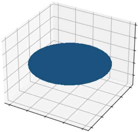
Since we are interested in point clouds, we can transform our meshes into points via the usage of torch_geometric.transforms.
In particular, PyG provides the SamplePoints transformation, which will uniformly sample a fixed number of points on the mesh faces according to their face area.
We can add this transformation to the dataset by simply setting it via dataset.transform = SamplePoints(num=...).
Each time an example is accessed from the dataset, the transformation procedure will get called, converting our mesh into a point cloud.
Note that sampling points is stochastic, and so you will receive a new point cloud upon every access:
import torch_geometric.transforms as T

dataset.transform = T.SamplePoints(num=256)

data = dataset[0]
print(data)
>>> Data(pos=[256, 3], y=[1])
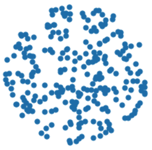
Note that we now have 256 points in our example, and the triangular connectivity stored in face has been removed.
Visualizing the points now shows that we have correctly sampled points on the surface of the initial mesh:
Finally, let’s convert our point cloud into a graph.
Since we are interested in learning local geometric structures, we want to construct a graph in such a way that nearby points are connected.
Typically, this is either done via \(k\)-nearest neighbor search or via ball queries (which connect all points that are within a certain radius to the query point).
PyG provides utilities for such graph generation via the KNNGraph and RadiusGraph transformations, respectively.
from torch_geometric.transforms import SamplePoints, KNNGraph

dataset.transform = T.Compose([SamplePoints(num=256), KNNGraph(k=6)])

data = dataset[0]
print(data)
>>> Data(pos=[256, 3], edge_index=[2, 1536], y=[1])
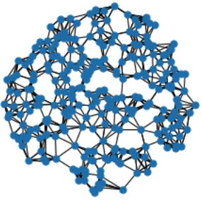
You can see that the data object now also contains an edge_index representation, holding 1536 edges in total, 6 edges for every of the 256 points.
We can confirm that our graph looks good via the following visualization:
PointNet++ Implementation
PointNet++ is a pioneering work that proposes a Graph Neural Network architecture for point cloud classification and segmentation. PointNet++ processes point clouds iteratively by following a simple grouping, neighborhood aggregation and downsampling scheme:
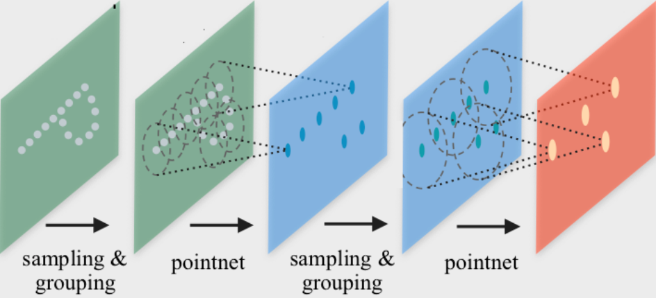
The grouping phase constructs a graph \(k\)-nearest neighbor search or via ball queries as described above.
The neighborhood aggregation phase executes a GNN layer that, for each point, aggregates information from its direct neighbors (given by the graph constructed in the previous phase). This allows PointNet++ to capture local context at different scales.
The downsampling phase implements a pooling scheme suitable for point clouds with potentially different sizes. Due to simplicity, we will ignore this phase for now. We recommend to take a look at examples/pointnet2_classification.py on guidance to how to implement this step.
Neighborhood Aggregation
The PointNet++ layer follows a simple neural message passing scheme defined via
where
\(\mathbf{h}_i^{(\ell)} \in \mathbb{R}^d\) denotes the hidden features of point \(i\) in layer \(\ell\), and
\(\mathbf{p}_i \in \mathbf{R}^3$\) denotes the position of point \(i\).
We can make use of the MessagePassing interface in PyG to implement this layer from scratch.
The MessagePassing interface helps us in creating message passing graph neural networks by automatically taking care of message propagation.
Here, we only need to define its message() function and which aggregation scheme we want to use, e.g., aggr="max" (see here for the accompanying tutorial):
from torch import Tensor
from torch.nn import Sequential, Linear, ReLU

from torch_geometric.nn import MessagePassing


class PointNetLayer(MessagePassing):
    def __init__(self, in_channels: int, out_channels: int):
        # Message passing with "max" aggregation.
        super().__init__(aggr='max')

        # Initialization of the MLP:
        # Here, the number of input features correspond to the hidden
        # node dimensionality plus point dimensionality (=3).
        self.mlp = Sequential(
            Linear(in_channels + 3, out_channels),
            ReLU(),
            Linear(out_channels, out_channels),
        )

    def forward(self,
        h: Tensor,
        pos: Tensor,
        edge_index: Tensor,
    ) -> Tensor:
        # Start propagating messages.
        return self.propagate(edge_index, h=h, pos=pos)

    def message(self,
        h_j: Tensor,
        pos_j: Tensor,
        pos_i: Tensor,
    ) -> Tensor:
        # h_j: The features of neighbors as shape [num_edges, in_channels]
        # pos_j: The position of neighbors as shape [num_edges, 3]
        # pos_i: The central node position as shape [num_edges, 3]

        edge_feat = torch.cat([h_j, pos_j - pos_i], dim=-1)
        return self.mlp(edge_feat)
As one can see, implementing the PointNet++ layer is quite straightforward in PyG.
In the __init__() function, we first define that we want to apply max aggregation, and afterwards initialize an MLP that takes care of transforming node features of neighbors and the spatial relation between source and destination nodes to a (trainable) message.
In the forward() function, we can start propagating messages based on edge_index, and pass in everything needed in order to create messages.
In the message() function, we can now access neighbor and central node information via *_j and *_i suffixes, respectively, and return a message for each edge.
Network Architecture
We can make use of above PointNetLayer to define our network architecture (or use its equivalent torch_geometric.nn.conv.PointNetConv directly integrated in PyG).
With this, our overall PointNet architecture looks as follows:
from torch_geometric.nn import global_max_pool


class PointNet(torch.nn.Module):
    def __init__(self):
        super().__init__()

        self.conv1 = PointNetLayer(3, 32)
        self.conv2 = PointNetLayer(32, 32)
        self.classifier = Linear(32, dataset.num_classes)

    def forward(self,
        pos: Tensor,
        edge_index: Tensor,
        batch: Tensor,
    ) -> Tensor:

        # Perform two-layers of message passing:
        h = self.conv1(h=pos, pos=pos, edge_index=edge_index)
        h = h.relu()
        h = self.conv2(h=h, pos=pos, edge_index=edge_index)
        h = h.relu()

        # Global Pooling:
        h = global_max_pool(h, batch)  # [num_examples, hidden_channels]

        # Classifier:
        return self.classifier(h)


model = PointNet()
If we inspect the model, we can see the everything is initialized correctly:
print(model)
>>> PointNet(
...   (conv1): PointNetLayer()
...   (conv2): PointNetLayer()
...   (classifier): Linear(in_features=32, out_features=40, bias=True)
... )
Here, we create our network architecture by inheriting from torch.nn.Module and initialize two PointNetLayer modules and a final linear classifier in its constructor.
In the forward() method, we apply two graph-based convolutional operators and enhance them by ReLU non-linearities.
The first operator takes in 3 input features (the positions of nodes) and maps them to 32 output features.
After that, each point holds information about its 2-hop neighborhood, and should already be able to distinguish between simple local shapes.
Next, we apply a global graph readout function, i.e., global_max_pool(), which takes the maximum value along the node dimension for each example.
In order to map the different nodes to their corresponding examples, we use the batch vector which will be automatically created for use when using the mini-batch torch_geometric.loader.DataLoader.
Last, we apply a linear classifier to map the global 32 features per point cloud to one of the 40 classes.
Training Procedure
We are now ready to write two simple procedures to train and test our model on the training and test datasets, respectively. If you are not new to PyTorch, this scheme should appear familiar to you. Otherwise, the PyTorch documentation provide a good introduction on how to train a neural network in PyTorch:
from torch_geometric.loader import DataLoader

train_dataset = GeometricShapes(root='data/GeometricShapes', train=True)
train_dataset.transform = T.Compose([SamplePoints(num=256), KNNGraph(k=6)])
test_dataset = GeometricShapes(root='data/GeometricShapes', train=False)
test_dataset.transform = T.Compose([SamplePoints(num=256), KNNGraph(k=6)])

train_loader = DataLoader(train_dataset, batch_size=10, shuffle=True)
test_loader = DataLoader(test_dataset, batch_size=10)

model = PointNet()
optimizer = torch.optim.Adam(model.parameters(), lr=0.01)
criterion = torch.nn.CrossEntropyLoss()

def train():
    model.train()

    total_loss = 0
    for data in train_loader:
        optimizer.zero_grad()
        logits = model(data.pos, data.edge_index, data.batch)
        loss = criterion(logits, data.y)
        loss.backward()
        optimizer.step()
        total_loss += float(loss) * data.num_graphs

    return total_loss / len(train_loader.dataset)


@torch.no_grad()
def test():
    model.eval()

    total_correct = 0
    for data in test_loader:
        logits = model(data.pos, data.edge_index, data.batch)
        pred = logits.argmax(dim=-1)
        total_correct += int((pred == data.y).sum())

    return total_correct / len(test_loader.dataset)

for epoch in range(1, 51):
    loss = train()
    test_acc = test()
    print(f'Epoch: {epoch:02d}, Loss: {loss:.4f}, Test Acc: {test_acc:.4f}')
Using this setup, you should get around 75%-80% test set accuracy, even when training only on a single example per class.